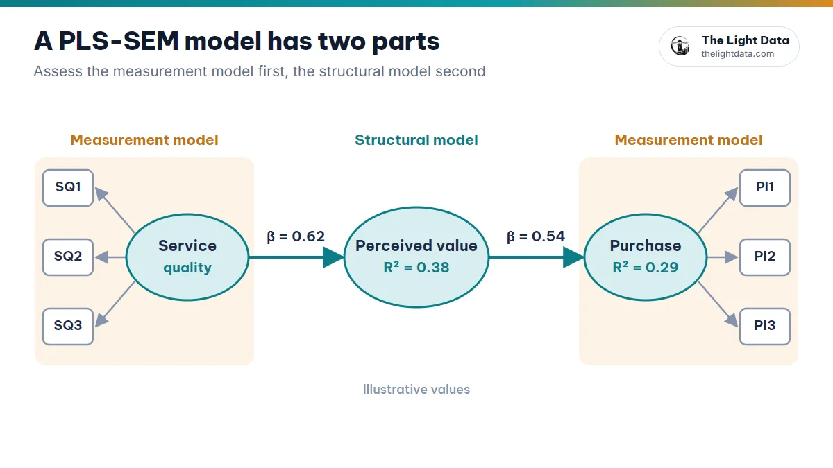
Your scales pass, you run bootstrapping, and out come table after table: Path Coefficients, T Statistics, P Values, R Square, f Square… Which hypotheses are supported? How do you write the conclusion? And what if your favorite hypothesis comes back with a P value of 0.21? This guide covers assessing a structural model in SmartPLS per Hair et al. (2022): reading the 9 indicators correctly, building your hypothesis table and handling unexpected results honestly.
① Check collinearity (VIF) → ② explanatory and predictive power (R², f², Q²) → ③ test the hypotheses (β, T and P from bootstrapping).
1VIF: checking collinearity in the structural model
Collinearity arises when predictors of the same dependent variable correlate too strongly with each other, which distorts the path coefficients. SmartPLS calculates VIF for each set of predictors pointing at one dependent variable.
| Predictor → Purchase Intention | VIF |
|---|---|
| Perceived value (PV) | 1.84 |
| Trust (TR) | 2.12 |
| Service quality (SQ) | 2.45 |
All are below 3, so there is no collinearity problem.
- VIF < 3: Ideal
- 3 ≤ VIF < 5: A possible problem; keep an eye on it
- VIF ≥ 5: Critical collinearity
2R²: what is a good value?
R² is the share of variance in the dependent variable explained by its predictors.
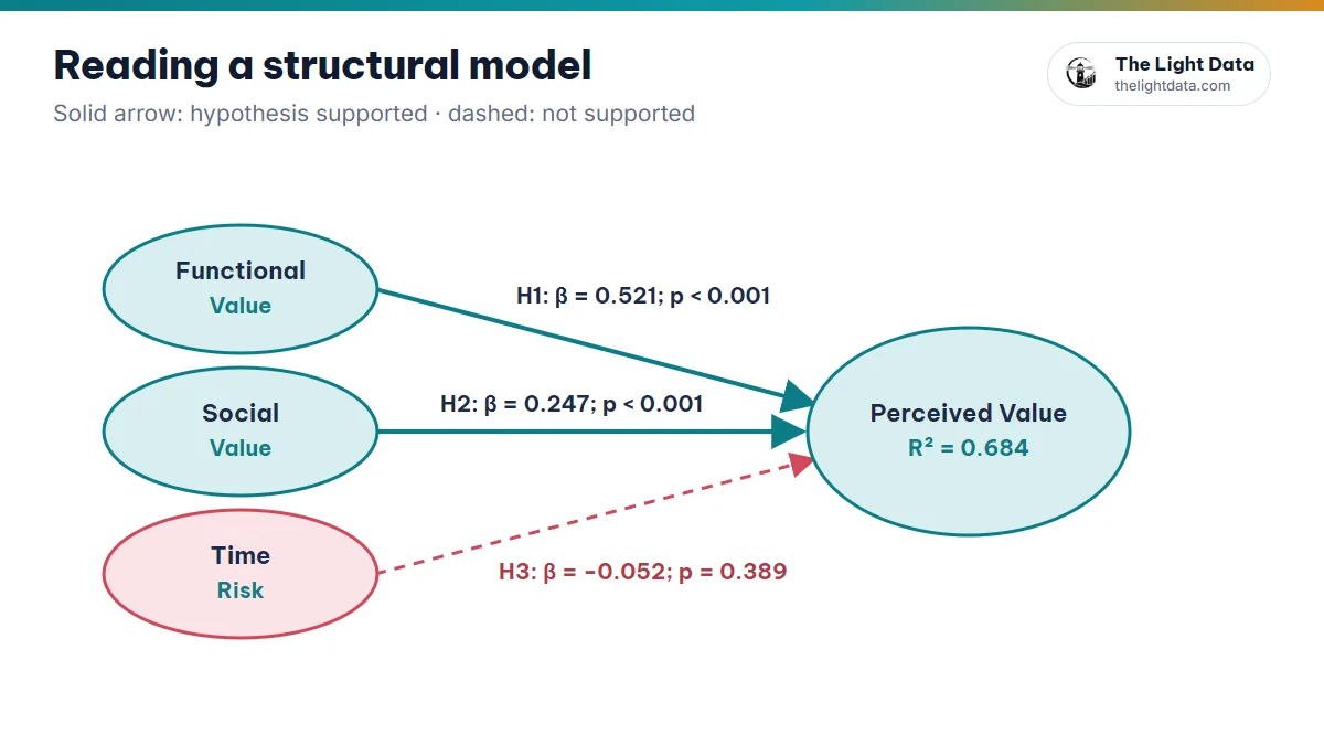
Functional, Social and Environmental Value explain Perceived Value with R² = 0.684: 68.4% of the variance is explained and 31.6% comes from factors outside the model.
- 0.75: Substantial
- 0.50: Moderate
- 0.25: Weak
These levels are only a guide. Hair et al. (2022) note that in consumer behavior research, an R² of around 0.20 can already be considered high. Compare with studies in your own field.
3Adjusted R²
A version of R² that accounts for the number of predictors, since adding any variable raises R² even if it means nothing.
R² = 0.705 and adjusted R² = 0.697 (a gap of 0.008): the predictors all contribute. With R² = 0.72 but adjusted R² = 0.54, the model may carry surplus variables.
4f²: which predictor has the strongest effect?
From Cohen (1988), f² measures each predictor’s own contribution to the dependent variable’s R², by comparing R² with and without it.
| Path | f² |
|---|---|
| PV → PI | 0.42 |
| Social Value → PV | 0.18 |
| Physical Risk → PV | 0.04 |
PV → PI is a large effect, Social Value medium and Physical Risk small.
- 0.02: Small
- 0.15: Medium
- 0.35: Large
5Q²: the model’s predictive power
R² tells you how well the model explains the data you have; Q² tells you how well it predicts. In SmartPLS 3, the Stone–Geisser Q² comes from blindfolding; SmartPLS 4 assesses predictive power with Q²predict through the PLSpredict procedure.
| Endogenous construct | Q² |
|---|---|
| Perceived Value | 0.412 |
| Purchase Intention | 0.327 |
Both are above 0, so the model has predictive relevance.
- Q² > 0: Predictive relevance (0.25 and 0.50 mark medium and large)
- Q² ≤ 0: No predictive relevance
6Paths: your hypotheses
Each arrow between two constructs is one hypothesis to test.
- H1: Functional Value → Perceived Value
- H2: Social Value → Perceived Value
- H3: Perceived Value → Purchase Intention
7Path coefficients (β): direction and strength
Standardized regression coefficients from −1 to +1: the sign gives the direction and the absolute value the strength.
| Path | β |
|---|---|
| Functional Value → PV | 0.521 |
| Social Value → PV | 0.247 |
| Physical Risk → PV | -0.184 |
A strong positive effect, a weaker positive effect and a negative effect.
8T statistics, from bootstrapping
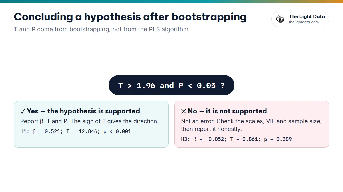
T statistics come from bootstrapping and test whether β differs significantly from 0. Note that the PLS algorithm gives no T or P values, so bootstrapping is essential (Hair et al., 2022 recommend 10,000 samples for final results).
- T > 1.645: Significant at the 10% level
- T > 1.96: Significant at the 5% level
- T > 2.576: Significant at the 1% level
9P values: is the hypothesis supported?
The P value is the probability of seeing a result at least this extreme if the null hypothesis (H₀: β = 0) were true. The smaller it is, the stronger the evidence for your hypothesis.
- P < 0.05: Significant; the hypothesis is supported
- P < 0.01 / < 0.001: Highly / very highly significant
- P ≥ 0.05: Not statistically significant
10Building the hypothesis table
| Hypothesis | β | T | P | Conclusion |
|---|---|---|---|---|
| H1: FV → PV | 0.521 | 12.846 | <0.001 | Supported |
| H2: SV → PV | 0.247 | 4.963 | <0.001 | Supported |
| H3: TR → PV | -0.052 | 0.861 | 0.389 | Not supported |
“Functional value has a positive effect on perceived value (β = 0.521; T = 12.846; p < .001), so hypothesis H1 is supported.” Write “p < .001” rather than “p = .000”.
11P value above 0.05: what now?
An unsupported hypothesis is not an error. It is a finding. Before you conclude, check:
- The measurement model: does it pass (AVE, HTMT)? Weak scales weaken coefficients.
- Collinearity: a high VIF can “share out” an effect among predictors.
- Sample size: do you have enough power for a small effect?
- Indirect effects: the variable may work through a mediator rather than directly.
- Context: sample characteristics, culture and timing may differ from the original study.
Do not add, remove or edit responses to make a P value look better. A committee will value a convincing discussion of why a hypothesis was not supported over a table of nothing but “supported”.
12Testing mediation in SmartPLS
After bootstrapping, look at Specific Indirect Effects. An indirect effect is significant when P < 0.05 (the 95% confidence interval excludes 0). Then compare it with the direct effect:
- Indirect significant, direct not significant → full mediation.
- Both significant → partial mediation.
- Indirect not significant → no mediation.
Plan your results chapter before you have data
On The Light Data’s model canvas, draw your model with positive and negative hypotheses and moderators, pick SmartPLS and read the path coefficients, bootstrap and R² tables on simulated data. It helps you picture how to present your results. Simulated data is for learning only and never replaces real data.
- VIF < 3 · compare R² and Q² with your field · f² shows which predictor is strongest.
- β gives direction and strength · T > 1.96 and P < 0.05 means the hypothesis is supported.
- T and P come from bootstrapping; P > 0.05 is a finding to discuss, not an error.